3.5. 多層パーセプトロン

XORを実装するためには, AND, NAND, ORゲートを組み合わせなければならない。

入力を \(x_1\), \(x_2\), NANDの出力を \(s_1\), ORの出力を \(s_2\) とすると、\(s_1\), \(s_2\)を入力としたANDの出力 \(y\) は以下の表の通りになる:

\(x_1\)	\(x_2\)	\(s_1\)	\(s_2\)	\(y\)
\(0\)	\(0\)	\(1\)	\(0\)	\(0\)
\(1\)	\(0\)	\(1\)	\(1\)	\(1\)
\(0\)	\(1\)	\(1\)	\(1\)	\(1\)
\(1\)	\(1\)	\(0\)	\(1\)	\(0\)

では、前に作成したNAND, ORを使用して、XORの結果を出力する関数を作成しよう。

import numpy as np
from matplotlib import pyplot as plt

def AND(x1, x2):
    """
    AND関数

    Parameters
    ----------
    x1 : float
        入力1
    x2 : float
        入力2
    """
    x = np.array([x1, x2])
    w = np.array([0.5, 0.5])
    b = -0.7
    tmp = np.sum(w * x) + b
    if tmp <= 0:
        return 0
    else:
        return 1

def NAND(x1, x2):
    """
    NAND関数

    Parameters
    ----------
    x1 : float
        入力1
    x2 : float
        入力2
    """
    x = np.array([x1, x2])
    w = np.array([-0.5, -0.5])
    b = 0.7
    tmp = np.sum(w * x) + b
    if tmp <= 0:
        return 0
    else:
        return 1

def OR(x1, x2):
    """
    OR関数

    Parameters
    ----------
    x1 : float
        入力1
    x2 : float
        入力2
    """
    x = np.array([x1, x2])
    w = np.array([0.5, 0.5])
    b = -0.2
    tmp = np.sum(w * x) + b
    if tmp <= 0:
        return 0
    else:
        return 1

3.5.1. XORゲートの実装

def XOR(x1, x2):
    """
    XOR関数

    Parameters
    ----------
    x1 : float
        入力1
    x2 : float
        入力2
    """
    s1 = NAND(x1, x2)
    s2 = OR(x1, x2)
    return AND(s1, s2)

XOR(0, 0)

0

XOR(1, 0)

1

XOR(0, 1)

1

XOR(1, 1)

0

このように、複数のパーセプトロンを組み合わせたパーセプトロンのことを 多層パーセプトロン という。

XORは、NAND, ORの出力とANDの出力の組み合わせなので、2層のパーセプトロンである。 (本によっては、入力\(x_1\), \(x_2\)も入れて3層とすることもある)

3.5.2. 🤔XORをグラフにすると？

import numpy as np
from matplotlib import pyplot as plt
import itertools

if __name__ == "__main__":
    xs = np.array([[0, 0],
                   [1, 0],
                   [0, 1],
                   [1, 1]], dtype=np.float32)      # データ



    w = np.array([0, 0], dtype=np.float32)  # 重み
    b = 0  # バイアス
    lr = 0.01  # 学習率

    def predict(x):
        u = np.dot(x, w) - b
        return np.where(u > 0, 1, 0)

    # グラフの描画 from https://teratail.com/questions/177319
    fig, ax = plt.subplots()
    ax.set_xticks([0, 1]), ax.set_yticks([0, 1])
    ax.set_xlim(-0.5, 1.5), ax.set_ylim(-0.5, 1.5)

    # サンプルを描画する。
    ax.scatter(xs[:, 0], xs[:, 1], s=30)

    # 各点の推論結果を得る。
    X, Y = np.meshgrid(np.linspace(*ax.get_xlim(), 100),
                       np.linspace(*ax.get_ylim(), 100))
    XY = np.column_stack([X.ravel(), Y.ravel()])
    Z = np.array([XOR(x[0], x[1]) for x in XY]).reshape(X.shape)

    # 等高線を描画する。
    ax.contourf(X, Y, Z, alpha=0.4, cmap='RdBu')

    plt.show()

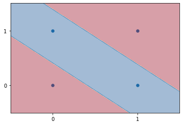
曲線にならなかったね…