3.4. パーセプトロンの限界

XORゲート

\(x_1\)	\(x_2\)	\(y\)
\(0\)	\(0\)	\(0\)
\(1\)	\(0\)	\(1\)
\(0\)	\(1\)	\(1\)
\(1\)	\(1\)	\(0\)

XORゲートは、単体のパーセプトロンでは実現できない。その理由をグラフで見てみよう。

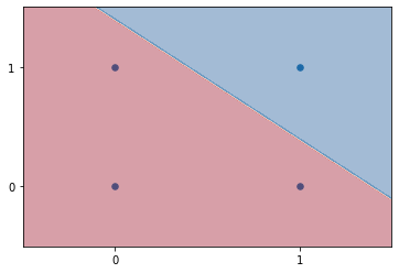
3.4.1. ANDのグラフ

import numpy as np
from matplotlib import pyplot as plt
import itertools

def AND(x1, x2):
    """
    AND関数

    Parameters
    ----------
    x1 : float
        入力1
    x2 : float
        入力2
    """
    x = np.array([x1, x2])
    w = np.array([0.5, 0.5])
    b = -0.7
    tmp = np.sum(w * x) + b
    if tmp <= 0:
        return 0
    else:
        return 1

if __name__ == "__main__":
    xs = np.array([[0, 0],
                   [1, 0],
                   [0, 1],
                   [1, 1]], dtype=np.float32)      # データ



    w = np.array([0, 0], dtype=np.float32)  # 重み
    b = 0  # バイアス
    lr = 0.01  # 学習率

    def predict(x):
        u = np.dot(x, w) - b
        return np.where(u > 0, 1, 0)

    # グラフの描画 from https://teratail.com/questions/177319
    fig, ax = plt.subplots()
    ax.set_xticks([0, 1]), ax.set_yticks([0, 1])
    ax.set_xlim(-0.5, 1.5), ax.set_ylim(-0.5, 1.5)

    # サンプルを描画する。
    ax.scatter(xs[:, 0], xs[:, 1], s=30)

    # 各点の推論結果を得る。
    X, Y = np.meshgrid(np.linspace(*ax.get_xlim(), 100),
                       np.linspace(*ax.get_ylim(), 100))
    XY = np.column_stack([X.ravel(), Y.ravel()])
    Z = np.array([AND(x[0], x[1]) for x in XY]).reshape(X.shape)

    # 等高線を描画する。
    ax.contourf(X, Y, Z, alpha=0.4, cmap='RdBu')

    plt.show()

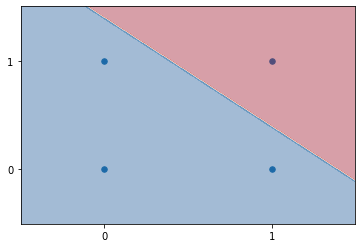
3.4.2. NANDのグラフ

import numpy as np
from matplotlib import pyplot as plt
import itertools

def NAND(x1, x2):
    """
    NAND関数

    Parameters
    ----------
    x1 : float
        入力1
    x2 : float
        入力2
    """
    x = np.array([x1, x2])
    w = np.array([-0.5, -0.5])
    b = 0.7
    tmp = np.sum(w * x) + b
    if tmp <= 0:
        return 0
    else:
        return 1

if __name__ == "__main__":
    xs = np.array([[0, 0],
                   [1, 0],
                   [0, 1],
                   [1, 1]], dtype=np.float32)      # データ



    w = np.array([0, 0], dtype=np.float32)  # 重み
    b = 0  # バイアス
    lr = 0.01  # 学習率

    def predict(x):
        u = np.dot(x, w) - b
        return np.where(u > 0, 1, 0)

    # グラフの描画 from https://teratail.com/questions/177319
    fig, ax = plt.subplots()
    ax.set_xticks([0, 1]), ax.set_yticks([0, 1])
    ax.set_xlim(-0.5, 1.5), ax.set_ylim(-0.5, 1.5)

    # サンプルを描画する。
    ax.scatter(xs[:, 0], xs[:, 1], s=30)

    # 各点の推論結果を得る。
    X, Y = np.meshgrid(np.linspace(*ax.get_xlim(), 100),
                       np.linspace(*ax.get_ylim(), 100))
    XY = np.column_stack([X.ravel(), Y.ravel()])
    Z = np.array([NAND(x[0], x[1]) for x in XY]).reshape(X.shape)

    # 等高線を描画する。
    ax.contourf(X, Y, Z, alpha=0.4, cmap='RdBu')

    plt.show()

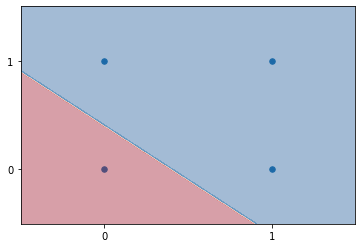
3.4.3. ORのグラフ

import numpy as np
from matplotlib import pyplot as plt
import itertools

def OR(x1, x2):
    """
    OR関数

    Parameters
    ----------
    x1 : float
        入力1
    x2 : float
        入力2
    """
    x = np.array([x1, x2])
    w = np.array([0.5, 0.5])
    b = -0.2
    tmp = np.sum(w * x) + b
    if tmp <= 0:
        return 0
    else:
        return 1

if __name__ == "__main__":
    xs = np.array([[0, 0],
                   [1, 0],
                   [0, 1],
                   [1, 1]], dtype=np.float32)      # データ



    w = np.array([0, 0], dtype=np.float32)  # 重み
    b = 0  # バイアス
    lr = 0.01  # 学習率

    def predict(x):
        u = np.dot(x, w) - b
        return np.where(u > 0, 1, 0)

    # グラフの描画 from https://teratail.com/questions/177319
    fig, ax = plt.subplots()
    ax.set_xticks([0, 1]), ax.set_yticks([0, 1])
    ax.set_xlim(-0.5, 1.5), ax.set_ylim(-0.5, 1.5)

    # サンプルを描画する。
    ax.scatter(xs[:, 0], xs[:, 1], s=30)

    # 各点の推論結果を得る。
    X, Y = np.meshgrid(np.linspace(*ax.get_xlim(), 100),
                       np.linspace(*ax.get_ylim(), 100))
    XY = np.column_stack([X.ravel(), Y.ravel()])
    Z = np.array([OR(x[0], x[1]) for x in XY]).reshape(X.shape)

    # 等高線を描画する。
    ax.contourf(X, Y, Z, alpha=0.4, cmap='RdBu')

    plt.show()

3.4.4. 何が言いたいのか

単体のパーセプトロンは、1本の直線として表現が可能なものしか分けることができない。

XOR は曲線になる。